Let's go through a step-by-step
process of ETL Operation using Fivetran connectors to Snowflake, DBT
Transformations, and Exploration using Looker Studio.
A little overview of the
Data Pipeline:
Technology Stack:
Snowflake: Snowflake is
the leading data warehouse built for the cloud. Its unique architecture
delivers proven breakthroughs in performance, concurrency, and simplicity. For
the first time, multiple groups can access petabytes of data at the same time,
up to 200 times faster and 10 times less expensive than solutions not built for
the cloud. Snowflake is a fully managed service with a pay-as-you-go model that
works on structured and semi-structured data.
Fivetran: Shaped by the
real-world needs of data analysts, Fivetran technology is the smartest, fastest
way to replicate your applications, databases, events, and files into a
high-performance cloud warehouse. Fivetran connectors deploy in minutes,
require zero maintenance, and automatically adjust to source changes; so, your
data team can stop worrying about engineering and focus on driving insights.
dbt: dbt is a
development environment built and maintained by Fishtown Analytics that speaks
the preferred language of data analysts everywhere SQL. With dbt, analysts take
ownership of the entire analytics engineering workflow, from writing data
transformation code to deployment and documentation.
Looker: Looker is a modern platform for data
that offers data analytics and business insights to every department at scale
and easily integrates into applications to deliver data directly into the
decision-making process.
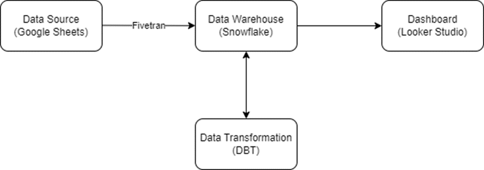
The following figure shows the Fivetran, dbt, and, Snowflake pipelines.

Data
Pipeline:
It starts with developing a Python script to establish a Fivetran
connector, facilitating the seamless connection of Google Sheets datasets to
the Snowflake warehouse.
Subsequently, the configuration of Snowflake with Data
Built Tools (DBT) is explored for optimal data management. SQL transformations
are then executed within the DBT environment, leading to the deployment of
refined models back into the Snowflake warehouse. The final stage involves
connecting the warehouse with Looker Studio, enabling the creation of dynamic
and interactive visualizations for comprehensive data analysis.
To do:
In this tutorial, we will be covering
different phases we completed in building our data pipeline:
Writing Python script
to create a Fivetran connector connecting datasets from Google Sheets to data
from our Snowflake warehouse.
Configuring Snowflake
with Data Built tools (DBT).
Writing SQL
transformation in DBT and deploying models back in our warehouse.
Connecting our warehouse
with Looker Studio and creating interactive visualizations.
About the dataset:
We download an open-source dataset
from Kaggle of sales data. It contained categories of each product with their
cost price and price each for which he sold each item, turnover, and quantity
ordered for each product in their category.
Each order is identified with its
unique order ID and the ordering date. The total dataset contained 185951 rows including headers.
Step 01: Creating Fivetran Connector using Python.
Fivetran provides us REST framework within Python to send
API calls to perform tasks. This can be found in their official API
documentation. In our code, we used POST calls with two predefined endpoints.
First, we used the ‘connector’
endpoint with configures defined in our payload variable. Then we used a sync
connector with that specified endpoint to sync our data.
It should be noted that the proper
API and other credentials are required which will be present in the Fivetran
user profile. Similarly, we configured our warehouse connection while creating
the Fivetran user profile to get specific credentials for proper connections
which will be further used in our code.
Code:
## Importing libraries |
|
import
requests |
from
requests.auth import HTTPBasicAuth |
import
json |
import
colorama |
from
colorama import Fore, Back, Style |
|
## Account Credentials | This will be obtained from the
API tab within the Fivetran Profile Account |
|
api_key
= '' |
api_secret
= '' |
a
= HTTPBasicAuth(api_key, api_secret) |
|
## Function for API calls |
|
def
atlas(method, endpoint, payload=None): |
|
base_url = 'https://api.fivetran.com/v1' |
h = { |
'Authorization':
f'Bearer {api_key}:{api_secret}' |
} |
url = f'{base_url}/{endpoint}' |
|
try: |
if
method == 'GET': |
response
= requests.get(url, headers=h, auth=a) |
elif
method == 'POST': |
response
= requests.post(url, headers=h, json=payload, auth=a) |
elif
method == 'PATCH': |
response
= requests.patch(url, headers=h, json=payload, auth=a) |
elif
method == 'DELETE': |
response
= requests.delete(url, headers=h, auth=a) |
else: |
raise
ValueError('Invalid
request method.') |
|
response.raise_for_status()
# Raise exception for 4xx or 5xx
responses |
|
return
response.json() |
except requests.exceptions.RequestException
as e: |
print(f'Request
failed: {e}') |
return
None |
|
## Creating our connector |
|
method
= 'POST' |
endpoint
= 'connectors' |
|
payload
= { |
"service":
"google_sheets", |
"group_id":
"", ##
Paste your group_id from the Fivetran Profile Data Tab |
"config":
{ |
"schema": "test_sheet_schema", |
"table": "test_sheet_table", |
"sheet_id": "", ##
Paste your google sheet link |
"named_range": "test_sheet_range", ##
Replace you selected named range within the google sheets |
"auth_type": "ServiceAccount" |
} |
} |
|
response
= atlas(method, endpoint, payload) |
|
print(response) |
|
## Sync data from sheet |
|
method
= 'POST' |
connector_id
= '' ##
Place your connector ID here from you Fivetran profile Setup tab |
endpoint
= f'connectors/{connector_id}/sync'
|
payload
= { |
"force":
False |
} |
|
response
= atlas(method, endpoint, payload) |
print(response) |
Step 02: Configuring Snowflake to DBT:
After having our dataset in our
snowflake warehouse, we configured our connection with DBT where we performed
our transformation. We followed the setup guide provided by DBT and pasted our
desired credentials to configure our DBT environment. DBT environments are
managed by version control git repositories that can either be localized or
personal based on the specific requirement.
In DBT, we linked our required
schema in the development environment and used the locally managed repository
by DBT itself to push our changes. We created branches for SQL models and
performed transformations which we pushed back into the repository and updated
the Snowflake warehouse.
Step 03: Writing SQL transformation in DBT:
The sales data included Quantity
Ordered, Price Each (the price at which each item was sold), Cost Price (the
cost of that item for the shopkeeper), Margin (profit on each item), Products,
and Categories, along with miscellaneous columns. As per this, we applied the
following transformations:
Our first transformation aimed to
obtain the total number of orders, total quantity ordered, and total turnover
for each item in their respective categories.
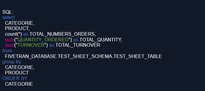
Our second transformation aimed to obtain the cost price, total turnover, and total profit, along with the profit percentage on each item in their respective categories.
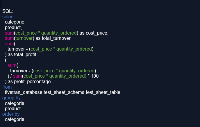
After a successful transformation,
we built our models and pushed back changes to our warehouse and the
DBT-managed repository.
Step 04: Exploration using Looker Studio:
Looker Studio is a BI tool within
Google Cloud that provides us flexibility in creating interactive dashboards
with various charts and exporting them in different templates. It not only
provides us good data exploration on our data but it also comes with various
connectors that enable us to connect to any data source and extract data tables
from pre-defined schemas.
We used one of these connectors to
connect to our snowflake warehouse where our previously transformed data was
present. After the correct configuration and successful connection, we fetched
data using SQL.

In the looker studio, we utilized
its toolkit to visualize our data in different formats.
First, we used the table kit to
paste a tabular representation of our overall data (in an interactive way) to
get a glimpse of the attributes present in our entire dataset. Then we plotted
a bar and pie chart that categorized the product categories concerning Cost
Price and Total turnover telling us how much is spent on each category and the
price on which it is sold as per the ordered quantity.
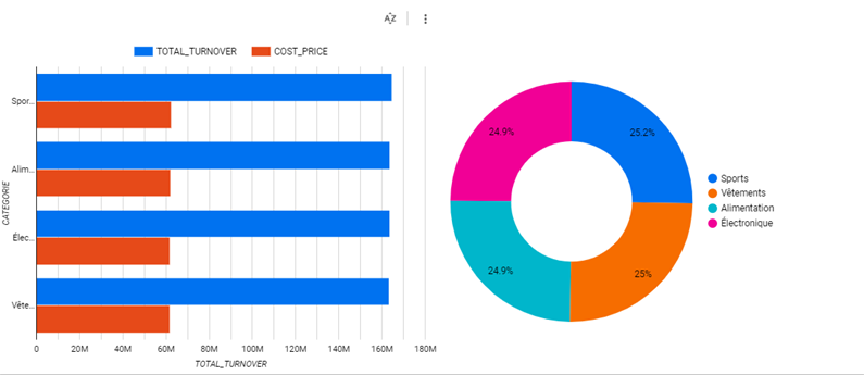
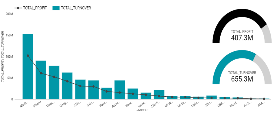
Then we moved towards the individual product since it linked with each category with one-to-many relation, and created interactive visualization covering the Bar-line chart for each product over cost price, turnover, a pie-chart with several orders on each product, and its heat tree map.
If
you have stayed with us till the end of the article, then feel free to share
your comments and read our other technological blogs.
Read more about Data
Pipelines: https://dotlabs.ai/blogs/2023/11/02/streamlining-data-pipelines-a-guide-to-etl-and-elt/

Dot Labs is an IT
outsourcing firm that offers a range of services, including software
development, quality assurance, and data analytics. With a team of skilled
professionals, Dot Labs offers nearshoring services to companies in North
America, providing cost savings while ensuring effective communication and
collaboration.
Visit our website: www.dotlabs.ai, for more information on how Dot
Labs can help your business with its IT outsourcing needs.
For more informative
Blogs on the latest technologies and trends click
here


